Bayesian inference for parameter estimation
Introduction
In this post we are going to describe how Bayesian statistics are used to model probabilistic phenomena. If you are new in statistics I recommend you to read a little about the differences between Bayesian and Frequentist approaches to inference—this for example. I must admit I felt quite confused at the beginning but if you want a brief summary about the differences, I would say that in the Frequentist school the parameters of the distribution are assumed to be fixed, while in the Bayesian they each (parameter) have another probability distribution associated to them—i.e. how probable is the given value of the parameter.
Imagine we have a set of events/data ($\mathcal{D}$) and we want to fit a probability distribution ($P$) to describe these events. First we have to pick a probability distribution, and second we need to estimate which are the paremeters ($\theta$) that fit the data the best.
Fitting the parameters can be done using Bayesian (or Frequentist) inference. Choosing the model will be up to you and the success of it will depend on your intuition.
Let’s start explaining Bayes’ formula:
\[\overbrace{P(\theta\mid \mathcal{D})}^\text{posterior} = \frac{\overbrace{P(\mathcal{D}\mid \theta)}^\text{likelihood}\times\overbrace{P(\theta)}^\text{prior}}{\underbrace{P(\mathcal{D})}_\text{Evidence or marginal likelihood}} \, , \qquad \, P(\mathcal{D}) = \int P(\mathcal{D}\mid \theta)P(\theta)\, d\theta\]In this formula we find two sets of variables that play a role:
- $\theta$ : represents the variables that we want to estimate from a predefined probability distribution—the mean and variance of a Gaussian for example.
- $\mathcal{D}$ : represents the observed data or events. We will use this data to estimate the parameters $\theta$.
Let’s put into words what each term in that equation means:
- $P(\theta \mid \mathcal{D})$ : Probability of $\theta$ being the true value given the data $\mathcal{D}$.
- $P( \mathcal{D} \mid \theta)$ : Probability of seeing the data $\mathcal{D}$ given the model parameters $\theta$.
- $P(\theta)$ : Probability that the model parameters $\theta$ being realized.
- $P(\mathcal{D})$ : Probability that the data is created by any of the possible models parametrized by $\theta$.
Example: tossing coins
The experiment is the following: someone is presented to us with a coin, a priori we do not know if the coin is biased or not, therefore we are going to throw the coin a number of times and see the results. From there we will be able to extract certain information and draw some conclusions. That is indeed how inference works, the main assumption is that there is an underlying—and unknown—probability distribution, let’s call it $P^*$, which we want to estimate. In order to do so you take several samples that come from this unknown distribution and try to fit a model $P$ which approximates its behaviour.
In order to model the coin tossing we are going to choose a Binomial distribution:
\[P(\mathcal{D}\mid \theta) = \binom{N_1}{n_1} \,\theta^{N_1-n_1}(1-\theta)^{n_1}\, ,\]which is a sensible choice given that the coin outputs are not correlated and are binary. In general this will be a choice of yours to decide which distribution $P(\mathcal{D}\mid \theta) $ fits best your phenomena. In this case the data is $\mathcal{D} = \{N_1,n_1\}$ where:
- $N_1$ : the number of times that we have flipped the coin,
- $n_1$ : the number of times we have got heads.
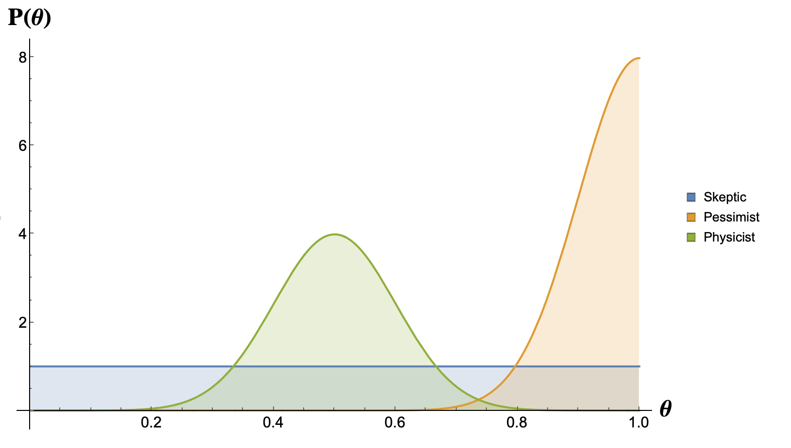
Now, our bias about the parameter $\theta$ (i.e. if we think the coin is fair or not) is encoded in the prior distribution $P(\theta)$. Let’s imagine that 3 players are going to play together against some adversary in the coin flipping game. One of the players is a pessimist so he thinks the coin is going to be clearly biased, another player is just highly skeptical and believes all possibilities are equally probable and a physicist who after examining carefully the coin he is quite confident the coin is fair.
\[P(\theta) = \begin{cases} 1 &\quad\text{Skeptic},\\[2mm] 2\cdot \mathcal{N}(1,0.1) &\quad\text{Pessimist}, \\[2mm] \mathcal{N}(0.5,0.1) &\quad\text{Physicist} \end{cases}\]Where $\mathcal{N}(\mu,\sigma)$ is the normal distribution. Remember that $\theta \in [0,1]$, therefore $P(\theta)$ is just defined in this range. Note that all the priors are normalized in the range $[0,1]$, i.e.
\[\int_0^1 P(\theta)\, d\theta = 1\, , \quad \text{For all players}\]Let’s plot the Priors for each case:

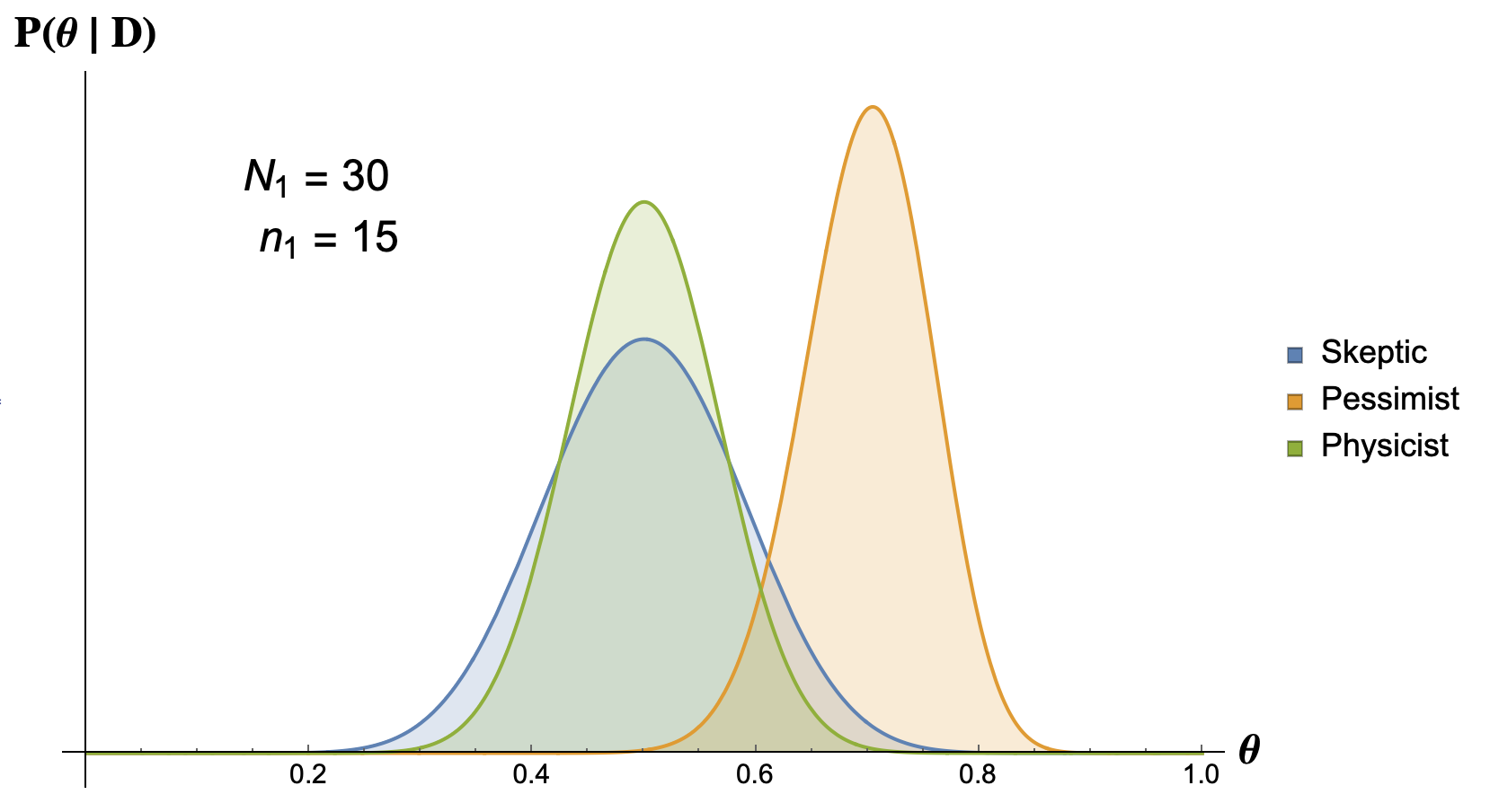
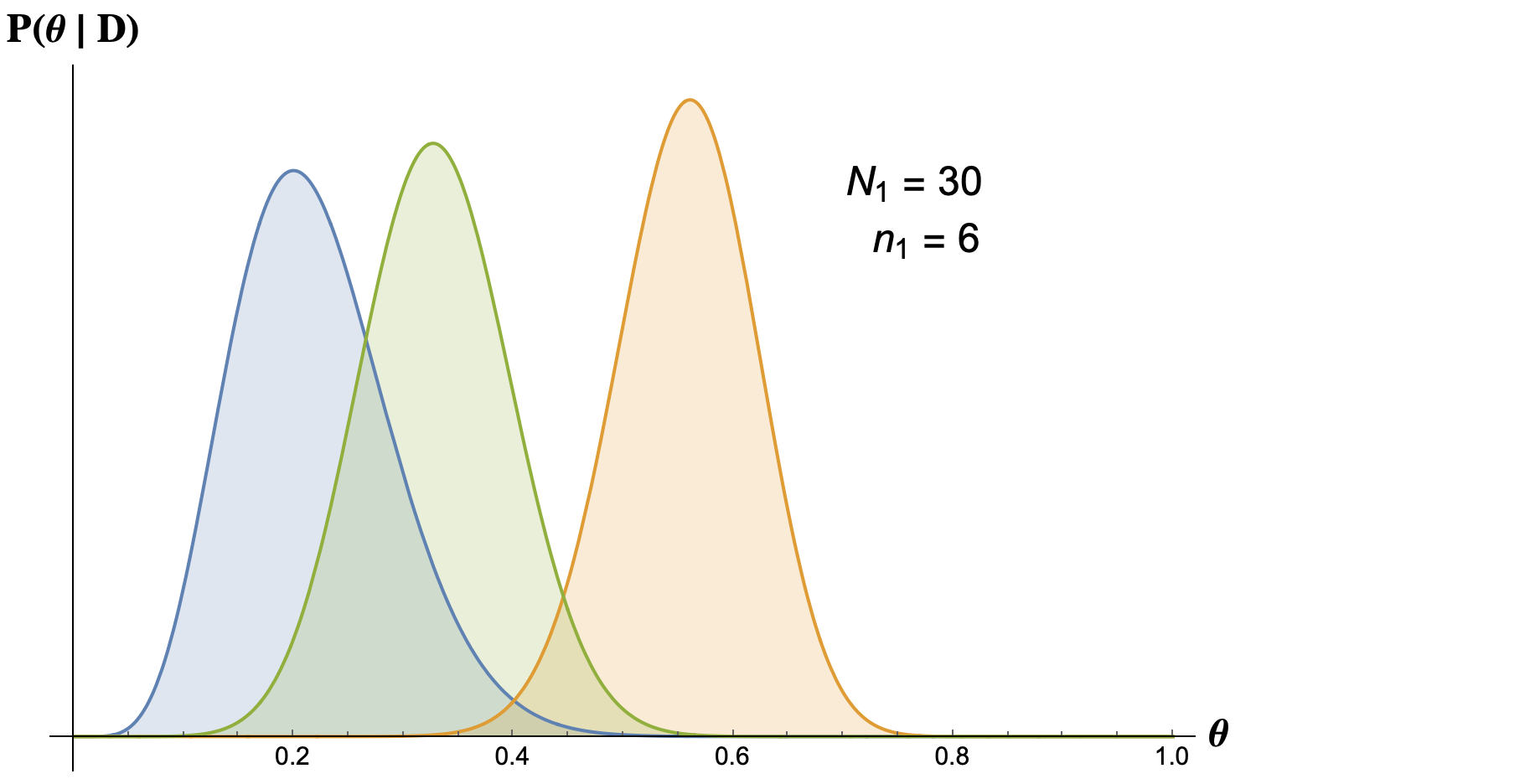
Now we flip the coin $N_1 = 30$ times and let’s see what happens to the posteriors for two different outcomes:
- Case one: 30 tosses, 15 heads,
- Case two: 30 tosses, 6 heads.


Case one: We see that when the data points to the case where the coin is fair, both the pysicist and the skeptic give the highest probability to $\theta = 1/2$. But there is a difference, which is the width of the distributions. As you can see the physicist has a narrower distribution around $\theta = 1/2$ meaning that he is more confident than the skeptic that the coin is fair. On the other hand the pessimist is still thinking that the coin is biased, he believes that the coin is not 100% biased but he does not have a high confidence that the true value of $\theta$ is $1/2$.
Case two: Here the skeptic believes that the true value of $\theta$ is $6/30=0.2$. The skeptic will always give the highest probability to $\theta$ to the frequency of heads in the data. On the other hand the physicist believes that the most probable value is now $0.32$ while the pessimist believes that the most probable value is $0.56$.
So always the data $\mathcal{D}$ updates the previous beliefs $P(\theta)$ of each of the players. Here you can see how the bias influences the posterior probability. But not so fast, you might feel a bit suspicious that the final outcome depends on the person who performs the experiment. After all, isn’t science based on the assumption that the results of experiments are independent on the person who carries them out? Well, Bayesian statistics have generated a lot of controversy and the fact that the prior is subjective is one of its main critics.
We can keep iterating this process. So our beliefs have been updated after observing the data. Now let’s assume we have a second step, we observe new data $\mathcal{D}_2 = \{N_2, n_2\}$. What we are going to do is use the updated beliefs $P(\theta\mid \mathcal{D}_1)$ as the prior for $\mathcal{D}_2$.
\[P(\theta \mid \mathcal{D}_2) = \frac{P(\mathcal{D}_2\mid \theta)\times P(\theta\mid \mathcal{D_1})}{P(\mathcal{D}_2)}\, , \qquad P(\mathcal{D}_2) = \int_0^1 P(\mathcal{D}_2\mid \theta)P(\theta\mid \mathcal{D_1}) \, d\theta\]As you can see you can keep updating your beliefs in the parameter $\theta$ every time that you observe new data. After $m$ iterations we would have:
\[P(\theta \mid \mathcal{D}_{m+1}) \propto P(\theta) \prod_{i = 1}^{m} P(\mathcal{D}_i\mid \theta) \equiv P(\theta) \mathcal{L}_m (\theta)\]Where the function $\mathcal{L}_m$ is the so-called likelihood function after $m$ samples of data have been observed.
So, in general after $m$ observations we will have:
\[P(\theta \mid \mathcal{D}_m, \ldots , \mathcal{D}_1) = \frac{P(\mathcal{D}_m, \ldots , \mathcal{D}_1\mid \theta)P(\theta)}{P(\mathcal{D}_1, \ldots , \mathcal{D}_m)}\]It is worth mentioning that in general:
\[\mathcal{L}_m (\theta) = P(\mathcal{D}_m, \ldots , \mathcal{D}_1\mid \theta) \neq \prod_{i = 1}^{m} P(\mathcal{D}_i\mid \theta)\]The last inequality just becomes equality when the events $\mathcal{D}_1,\ldots, \mathcal{D}_n$ are considered to be independent, which is a common assumption in the Machine Learning community.
If you wonder what the Frequentist approach to this problem would be, it is quite easy: the frequentist would look for the parameters $\hat{\theta}$ that maximize the probability of observing the data $\mathcal{D}_1, \ldots, \mathcal{D}_n$. This is known as Maximum Likelihood Estimation (MLE):
\[\hat{\theta} = \underset{\theta}{\operatorname{arg\;max}}\, \mathcal{L}_m (\theta)\]